Research article · Mathematics
Why randomness returns in 2D—but may escape in 3D
At each step, a walker randomly chooses one neighbouring direction. On a line and on a plane it returns to its starting point almost surely. In space there is a positive probability that it never returns. One extra dimension changes the answer.
One-sentence conclusion
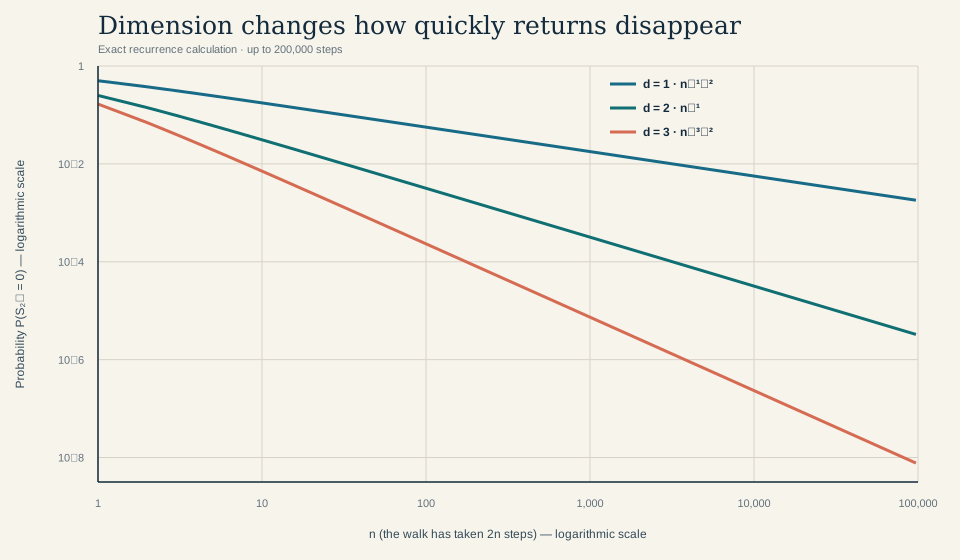
For simple symmetric random walk on , the probability of being at the origin after 2n steps decays as ; its sum diverges in dimensions 1 and 2 but converges from onward, exactly the criterion separating almost-sure return from possible escape.
1. The problem and precise definitions
The walk starts at on the integer lattice . At each time it adds, with equal probability, one of the 2d vectors : exactly one coordinate changes by one unit. Steps are independent. The model is “simple” because only nearest neighbours are allowed and “symmetric” because no direction is favoured.
The first return time is . The walk is recurrent if and transient if this probability is strictly below 1. “Almost surely” permits exceptional paths of probability zero and gives no maximum return time.
The question is therefore sharp: in which dimensions do the opportunities for return remain abundant enough to make a return certain? Pólya answered it in 1921: recurrence for ; transience for .[1][9]
2. Search and source selection
The search was conducted on 11 September 2026 across EuDML, DOI and publisher pages, the Dartmouth, Chicago and Duke author archives, and the Cambridge, Wiley and AMS catalogues. Queries combined “Pólya random walk recurrence”, “lattice Green function”, “local central limit theorem”, “Chung–Fuchs criterion”, “multiple returns” and “electric networks recurrence”.
Ten central references were retained: the original paper, the general Chung–Fuchs criterion, two historical works on lattice integrals and multiple returns, two classic monographs, three modern or pedagogical treatments, and one extension to infinite graphs. Popular accounts without proofs, irreproducible simulations and variants remote from were excluded.
Bibliographic pages were used to verify editions, DOIs and scope; fully accessible texts were used to check definitions, the Green-function equivalence, the asymptotic proof and the electrical analogy. No numerical result is borrowed from a third-party simulation.
3. From returns to expected visits
Set and . The quantity G, the Green function at the origin, is the expected number of visits to the origin including time zero. It adds the probabilities of being there at each exact time n; it does not assume that those events are independent.
Let , the probability of returning at least once. After every return, the Markov property restarts the same problem. The number of visits therefore has the geometric structure : if , then ; if , G diverges. Proving recurrence is thus exactly the same as testing whether diverges.[8][9]
This avoids a trap: divergence of does not generally justify a naïve Borel–Cantelli argument because return events are dependent. The Markov restart is what makes the equivalence exact here.
4. Why the threshold is two
The characteristic function of one step is . Fourier inversion gives . To sum safely, introduce and then let s tend to one: .[2][8]
The entire question concentrates near , where . Consequently, behaves like . The Green kernel therefore behaves like a constant divided by , where .
In radial coordinates, a shell of radius r contributes a volume factor proportional to . The decisive integral becomes . It diverges for and but converges for . By the previous equivalence, this is exactly the recurrence–transience threshold.
5. Reproducible calculation in dimensions 1–3
Returns are possible only at even times. In one dimension, . In two dimensions, the combinatorial identity yields the and decay rates. In three dimensions, an exact recurrence for multinomial coefficients computes without simulation.[4][5][9]
The script sums terms through , or 200,000 steps. For the partial sum is 1.514910606. A first-order local-central-limit tail correction gives and hence . The difference from the published constant 0.3405373296 is ; this agreement is a numerical check, not the proof of transience.[3][6][9]
| Total steps | |||
|---|---|---|---|
| 20 | 0.176197 | 0.0310454 | 0.00710835 |
| 2,000 | 0.0178390 | 0.000318230 | 0.00000737453 |
| 200,000 | 0.00178412 | 0.00000318309 | 0.00000000737727 |
6. Three intuitions to correct
- Almost-sure return does not mean quick return. In dimension two the sum diverges only logarithmically: returns become rare, but not fast enough for their total weight to remain finite.
- Recurrent does not mean confined. In dimensions one and two the walk reaches arbitrarily remote positions and still returns; the theorem concerns return, not bounded distance from the origin.
- Three recurrent coordinates do not make their coincidence recurrent. A three-dimensional return requires all three coordinates to be zero at the same time. That extra synchronisation changes the decay to , which is summable.
7. What the theorem does not say
- The proof targets a simple, symmetric, drift-free walk with independent steps on the integer lattice. Non-zero drift already makes a one-dimensional walk transient; heavy-tailed jumps can also alter the threshold.
- Euclidean dimension alone does not classify every graph. Volume growth, resistance, isoperimetry and global geometry can change recurrence; a graph drawn in the plane is not automatically recurrent.[2][10]
- The 200,000-step calculation uses exact recurrences in floating-point arithmetic and then an asymptotic tail extrapolation in dimension three. Its nine-decimal result is checked against the literature but is not presented as an interval-arithmetic certificate.
- The stated problem is nevertheless closed: for simple symmetric random walk on , the theorem and proof completely determine the answer. Open questions begin with other graphs, dependencies or step laws.
8. Central references actually consulted
Each note identifies the source’s role. Links point to the text, DOI or official publisher page.
G. Pólya (1921). Über eine Aufgabe der Wahrscheinlichkeitsrechnung betreffend die Irrfahrt im Straßennetz. Mathematische Annalen 84, 149–160.
The original paper establishing recurrence on one- and two-dimensional lattices and transience from dimension three onward.
K. L. Chung & W. H. J. Fuchs (1951). On the Distribution of Values of Sums of Random Variables. Memoirs of the American Mathematical Society, no. 6.
Generalises recurrence beyond the simple walk and underpins the characteristic-function criterion.
G. N. Watson (1939). Three Triple Integrals. Quarterly Journal of Mathematics os-10(1), 266–276.
Evaluates lattice integrals that enter the cubic lattice Green constant.
W. Feller (1968). An Introduction to Probability Theory and Its Applications, Volume I. 3rd ed., Wiley.
Reference for random walks, recurrent events, generating functions, and Stirling’s approximation.
C. Domb (1954). On Multiple Returns in the Random-Walk Problem. Proceedings of the Cambridge Philosophical Society 50(4), 586–591.
Connects fixed-time return probabilities with asymptotic methods and multiple returns.
E. W. Montroll (1956). Random Walks in Multidimensional Spaces, Especially on Periodic Lattices. Journal of the Society for Industrial and Applied Mathematics 4(4), 241–260.
Develops Green-function and return-probability calculations for several periodic lattices.
P. G. Doyle & J. L. Snell (1984/2006). Random Walks and Electric Networks. Carus Mathematical Monographs 22; open 2006 edition.
Gives a second reading of the dimensional threshold through effective resistance from the origin to infinity.
G. F. Lawler & V. Limic (2010). Random Walk: A Modern Introduction. Cambridge Studies in Advanced Mathematics 123.
Covers the local central limit theorem, Green functions, and the equivalence between recurrence and divergent expected visit counts.
R. Durrett (2019). Probability: Theory and Examples. 5th ed., Section 5.4.
Provides a modern combinatorial proof, the dimension-one-to-three asymptotics, and the numerical three-dimensional return constant.
W. Woess (2000). Random Walks on Infinite Graphs and Groups. Cambridge Tracts in Mathematics 138.
Shows why graph geometry, rather than its Euclidean drawing alone, governs recurrence beyond regular lattices.