Research article · Quantitative finance
Square-root-of-time: rule or shortcut?
Multiplying daily VaR by can feel almost automatic. Yet it is a theorem only under precise assumptions. We isolate them, then measure what happens when they stop holding.
One-sentence conclusion
The rule is exact for Gaussian VaR under independent returns with constant variance; elsewhere its error has no guaranteed sign or size, so risk should be modelled and validated directly at the target horizon.
1. The problem and definitions
Let be a portfolio’s log return on day t. Over h days, cumulative return is . Value at risk at 99%, written , is the loss threshold exceeded with 1% probability. A 3% VaR says nothing by itself about the average loss once 3% has been breached.
The square-root-of-time rule takes one-day VaR and sets . At ten days, the multiplier is . The question is not whether the arithmetic is convenient, but whether it preserves the loss-distribution quantile at the horizon actually being decided.
Both directions matter. Understatement leaves too little protection against loss; overstatement ties up capital unnecessarily or may reject an acceptable position. The sign of the error matters as much as its magnitude.
2. How the literature was selected
The search was performed on 4 September 2026 using publisher pages, DOI records, institutional archives and Bank for International Settlements documents. Queries combined “square-root-of-time”, “time scaling risk”, “temporal aggregation GARCH”, “interval forecast evaluation” and close variants.
Ten central texts were retained: foundational ARCH/GARCH papers, two studies directly about horizon scaling, one on temporal aggregation, a multi-day tail-risk method, a validation framework, a survey of stylised facts, a reference on VaR’s limitations, and the regulatory document that popularised . Secondary commentary, papers unrelated to horizon choice and duplicates were excluded.
The bibliography delineates what is known. Every number below comes solely from the stated formulae and simulations, not from a market dataset.
3. The case where is exact
Assume the are independent, identically distributed normal variables with zero mean and variance . Adding h independent normals gives , hence standard deviation . Because every centred-normal quantile is a fixed multiple of its standard deviation, .
Three properties do the work: zero cross-day covariance, unchanged variance, and a distribution family that remains shape-stable under addition. Independence without normality does not guarantee equality of finite-horizon quantiles; additive variance does not automatically imply identically scaled VaR.
4. Six reproducible stress tests
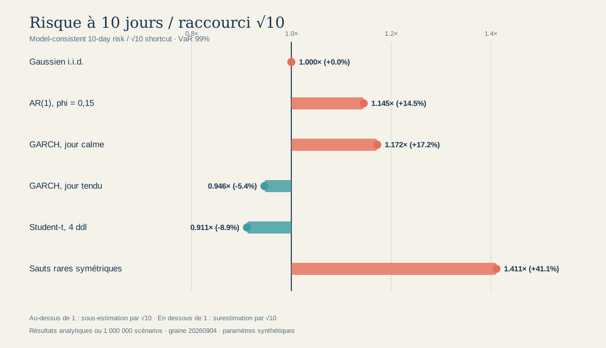
The protocol fixes trading days and 99% confidence. The first four results are analytical; the last two use 1,000,000 independent scenarios with seed 20260904. The ratio is model-consistent ten-day VaR divided by the shortcut. Above 1, understates risk; below 1, it overstates risk.
| Model | Ratio | Gap | Reading |
|---|---|---|---|
| i.i.d. Gaussian | 1.000× | 0.0% | Exact |
| AR(1), | 1.145× | +14.5% | Understatement |
| GARCH, calm day | 1.172× | +17.2% | Understatement |
| GARCH, stressed day | 0.946× | −5.4% | Overstatement |
| Student t, 4 df | 0.911× | −8.9% | Overstatement |
| Rare symmetric jumps | 1.411× | +41.1% | Understatement |
5. Why the error changes sign
Autocorrelation. For a stationary process, . The rule deletes every covariance term . With in our AR(1), they are positive: ten-day risk is 14.5% above the shortcut.
Conditional volatility. In the synthetic GARCH model, volatility reverts towards 1% with persistence . Starting from a calm 0.5% day makes too small because future variance rises: +17.2%. Starting from a stressed 2.5% day makes too large because it prolongs stress without mean reversion: −5.4%.
Heavy tails. Independent Student-t returns with four degrees of freedom are rescaled to 1% volatility. The one-day extreme quantile is heavy, while the ten-day sum begins to assume a less extreme shape; scaling the daily quantile overstates ten-day VaR here by 8.9%. This does not mean heavy tails make conservative in general.
Rare jumps. A 0.8% Gaussian diffusion receives a symmetric jump with total daily probability 0.5%. A daily 99% quantile misses the rarer jump; over ten days, the probability of at least one jump is about 4.9%. The quantile changes regime and understates simulated VaR by 41.1%.
6. A more defensible decision rule
Do not ban ; require evidence that it is admissible.
- Define the object first: portfolio, measure (VaR and preferably expected shortfall), confidence level, horizon, liquidation rule and units.
- Test the useful assumptions: return autocorrelation, dependence in squared or absolute returns, breaks, asymmetry and tail stability. No linear autocorrelation does not imply constant variance.
- Build a direct ten-day forecast: filtered simulation, conditional model, block-based historical scenarios or a suitable tail method. Fully revalue nonlinear positions.
- Compare with the direct model out of sample. Test both exceedance frequency and independence; clustered breaches reveal misspecified dynamics even when average frequency looks correct.
- Retain only if its error is bounded across relevant scenarios and the bound is compatible with the decision. Record the date, parameters and abandonment threshold.
7. Limitations and the open problem
- This is a mechanism demonstration, not an estimate for a real portfolio. Parameters were chosen to make effects legible; they describe no asset or historical period.
- One million scenarios reduce but do not remove Monte Carlo error. Student-t and jump ratios will move slightly under another seed. The JSON file distinguishes simulations from analytical identities.
- We cover additive returns and a linear exposure only. Options, liquidity, changing positions, multivariate dependence and expected shortfall can alter the result further.
- The general question—which aggregation model is best for a given portfolio—remains empirical. The defensible conclusion is narrower: is a model, not a universal law, and must be compared with a direct forecast of the target horizon.
8. Central references actually consulted
Each note states how the source enters the argument. Links point to the DOI, publisher or institutional archive.
Basel Committee on Banking Supervision (1995). An internal model-based approach to market risk capital requirements. Bank for International Settlements.
Historical regulatory source explicitly allowing one-to-ten-day √10 scaling and stating restrictions, notably for options.
R. F. Engle (1982). Autoregressive Conditional Heteroscedasticity with Estimates of the Variance of United Kingdom Inflation. Econometrica 50(4), 987–1007.
Foundational paper showing that a series may be uncorrelated while its conditional variance remains predictable.
T. Bollerslev (1986). Generalized Autoregressive Conditional Heteroskedasticity. Journal of Econometrics 31(3), 307–327.
Generalises ARCH and supplies the persistent-variance model used in one of our stress tests.
F. C. Drost & T. E. Nijman (1993). Temporal Aggregation of GARCH Processes. Econometrica 61(4), 909–927.
Shows that temporal aggregation changes GARCH parameters and is not equivalent to copying a daily variance.
F. X. Diebold, A. Hickman, A. Inoue & T. Schuermann (1997). Converting 1-Day Volatility to h-Day Volatility: Scaling by Root-h is Worse Than You Think. Wharton Financial Institutions Center Working Paper 97-34.
Directly studies horizon conversion and recommends models tailored to the horizon actually needed.
P. F. Christoffersen (1998). Evaluating Interval Forecasts. International Economic Review 39(4), 841–862.
Provides the conditional validation framework: correct exceedance frequency is insufficient if violations cluster.
P. Artzner, F. Delbaen, J.-M. Eber & D. Heath (1999). Coherent Measures of Risk. Mathematical Finance 9(3), 203–228.
Shows that VaR need not be subadditive and that a quantile does not summarise the full severity of the tail.
A. J. McNeil & R. Frey (2000). Estimation of Tail-Related Risk Measures for Heteroscedastic Financial Time Series: an Extreme Value Approach. Journal of Empirical Finance 7(3–4), 271–300.
Combines conditional volatility and extreme-value theory; its multi-day results outperform simple √h scaling.
R. Cont (2001). Empirical Properties of Asset Returns: Stylized Facts and Statistical Issues. Quantitative Finance 1(2), 223–236.
Surveys heavy tails, nonlinear dependence and volatility clustering across many markets.
J. Danielsson & J.-P. Zigrand (2006). On Time-Scaling of Risk and the Square-Root-of-Time Rule. Journal of Banking & Finance 30(10), 2701–2713.
Shows in a jump-diffusion model that the rule can systematically understate risk, increasingly at longer horizons and higher confidence levels.