HELIX-96 — turning 96 wells into a decision
An AI score ranks thousands of mutations. The question is not only what ranks first, but whether its probabilities travel to a new protein.
Reconstructed organization and AI score. Experimental effects from eight public ProteinGym assays; no clinical or human outcome.
5,600 public variants · synthetic scoreReading plan
From problem to decision
- 01
Understand the scarce resource
One plate, 96 experimental cavities and thousands of candidate variants.
- 02
Check the score
Separate already-known proteins from genuinely new proteins.
- 03
Correct confidence
Turn a score into a calibrated probability with uncertainty.
- 04
Organise the 96 experiments
Test 24 variants, retain a stop option, then use the remaining 72.
01
Before we begin
The problem
A reconstructed research team has a laboratory plate containing 96 small experimental wells to compare mutations proposed by a ranking model.
A protein is a chain of amino acids. Replacing one amino acid creates a variant; that change may improve, degrade or leave unchanged the measured biological function.
The reconstructed laboratory can test only 96 variants out of several thousand. A 96-well plate is a support containing 96 small cavities: each well hosts one distinct experiment here.
02
Phase 1
What the organization built
We begin by understanding the system as presented, without caricaturing it and before proposing any correction.
What the ranking engine does
The engine assigns each variant a score intended to reflect its chance of producing a positive experimental result. The organization ranks variants and considers filling the 96 wells with the highest scores.
To validate the engine, it randomly mixes variants and reserves a portion for testing. This random split often places mutations from the same protein in both training and test sets.
Why the first test is too easy
The model partly recognises features of proteins it has already seen. Good performance may therefore measure familiarity with those proteins rather than the ability to work on a new protein.
The corrected test removes one complete protein at a time. Results become much more dispersed: the score does not transport equally across biological contexts.
Initial approach summary
- Mutations are randomly separated between training and testing, separately for each biological experiment.
- Area under the ranking curve is 0.838 and squared probability error is 0.113: the result looks strong.
- But mutations from the same proteins appear on both sides, making the test too comfortable.
03
Phase 2
What the assessment checks and proposes
The second phase reproduces the mechanism, locates what breaks and turns criticism into a testable change.
Correct probability, not only ranking
Seven public groups estimate a shared relationship between score and outcome while allowing each group to depart from it. This hierarchical structure avoids treating eight biologically different experiments as identical.
Probability quality is measured with the Brier score: the squared gap between announced probability and observed outcome is computed. Lower values indicate better calibrated probabilities.
Create a stop option with 24 then 72 wells
Instead of committing all 96 experiments at once, the plan first uses 24 to check calibration on the new protein. A pre-specified rule may then stop, recalibrate or continue with the remaining 72 wells.
In this retrospective implementation, ranking does not change: one-shot and two-stage selections contain exactly the same 96 variants. The benefit is therefore the right to stop, not a demonstrated ranking gain.
Assessment
- When entire proteins are excluded from training, performance varies substantially across biological experiments.
- On the target group, nominal probabilities produce a Brier error of 0.215.
- The corrected selection achieves 47 positive results out of 96 versus 50 for the initial approach; no ranking gain is claimed.
Proposed correction
- Seven biological experiments learn a shared relationship between score and outcome, with a group-specific correction; the eighth remains the target.
- Four independent computational chains expose numerical stability and parameter uncertainty.
- Twenty-four experiments are read before deciding whether to stop, recalibrate or use the remaining 72, under a rule written in advance.
- Diversity rises from 64 to 69 unique positions.
04
Concepts and equations
No symbol without a definition
The same notes open from the “?” links placed throughout the article.
05
Numerical results
What the numbers actually measure
The four numbers summarise different questions: probability quality, numerical stability, actual effect of staging and positive-result count.
Brier score: nominal → hierarchical
Squared probability error; lower is better.
maximum R-hat diagnostic
Very close to 1: the four computational chains agree.
identical variants across both plans
One-shot and 24 + 72 plans retain the same list.
positive results: initial / corrected
The correction gains diversity, not positive-result count.
06 · See the evidence
Read the charts step by step
Each figure first explains how to read its axes and colours, then what it does—or does not—support.
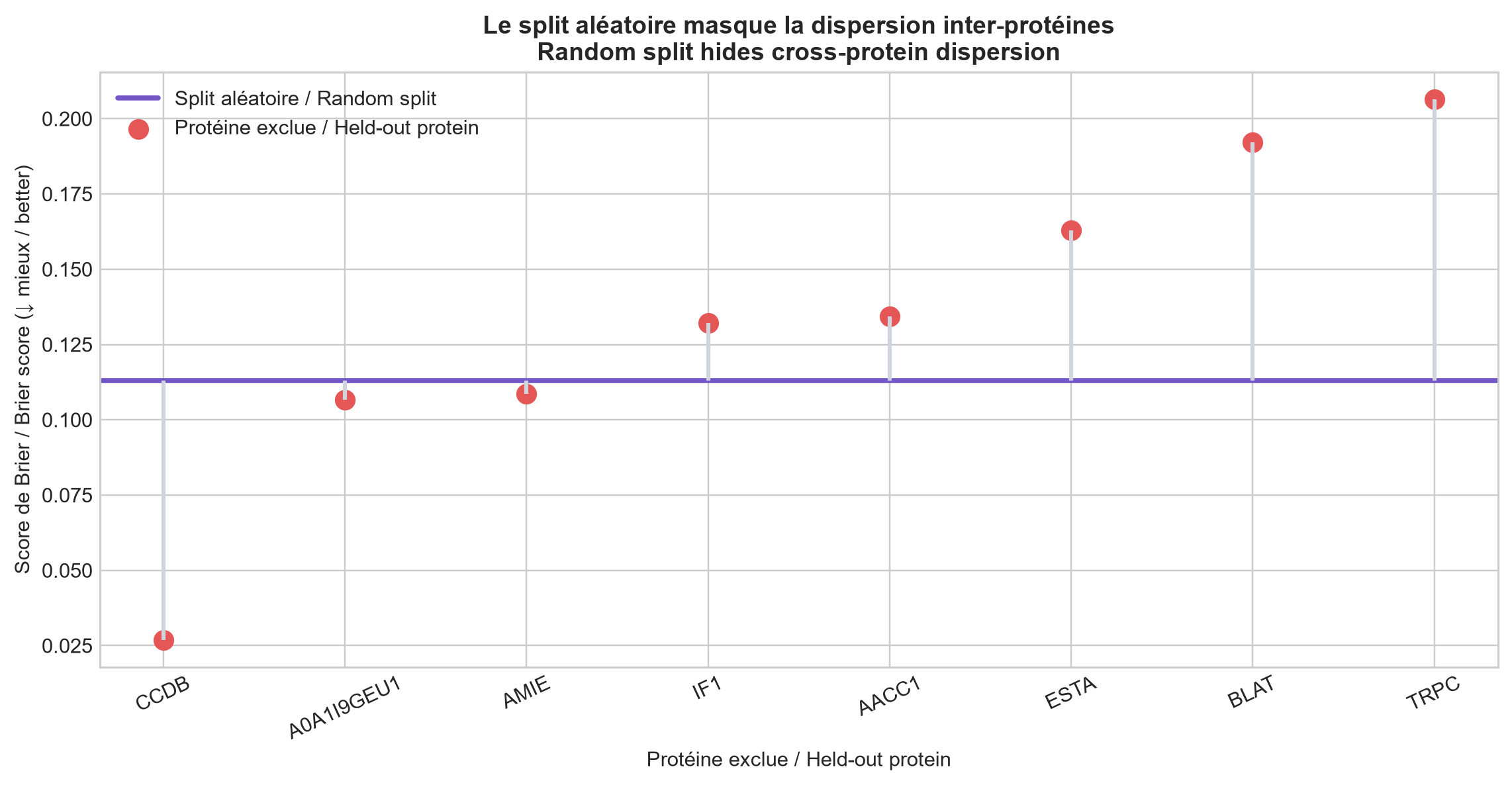
Gap between random separation and whole-protein-held-out validation
The figure has one panel. The horizontal axis lists eight proteins removed in turn from training; codes such as CCDB, A0A1I9GEU1 and TRPC are identifiers, not metrics. The vertical axis is Brier score, a unitless squared probability error: lower is better calibrated. The purple horizontal line near 0.113 is the result of a random split that mixes variants from the same proteins between training and test. Each red point is the score when the named protein is genuinely held out; the grey stem shows its gap from purple.
Protein-level results range from about 0.027 for CCDB to 0.206 for TRPC. Three proteins are at or below the random-split line, but five are above it, sometimes markedly so. We can conclude that a single random-split score hides substantial dispersion when transferring to an unseen protein. We cannot conclude that the purple line by itself quantifies one precise causal leakage mechanism, or that the values will recur on genuinely unseen data: the AI score is reconstructed from already-known public outcomes.
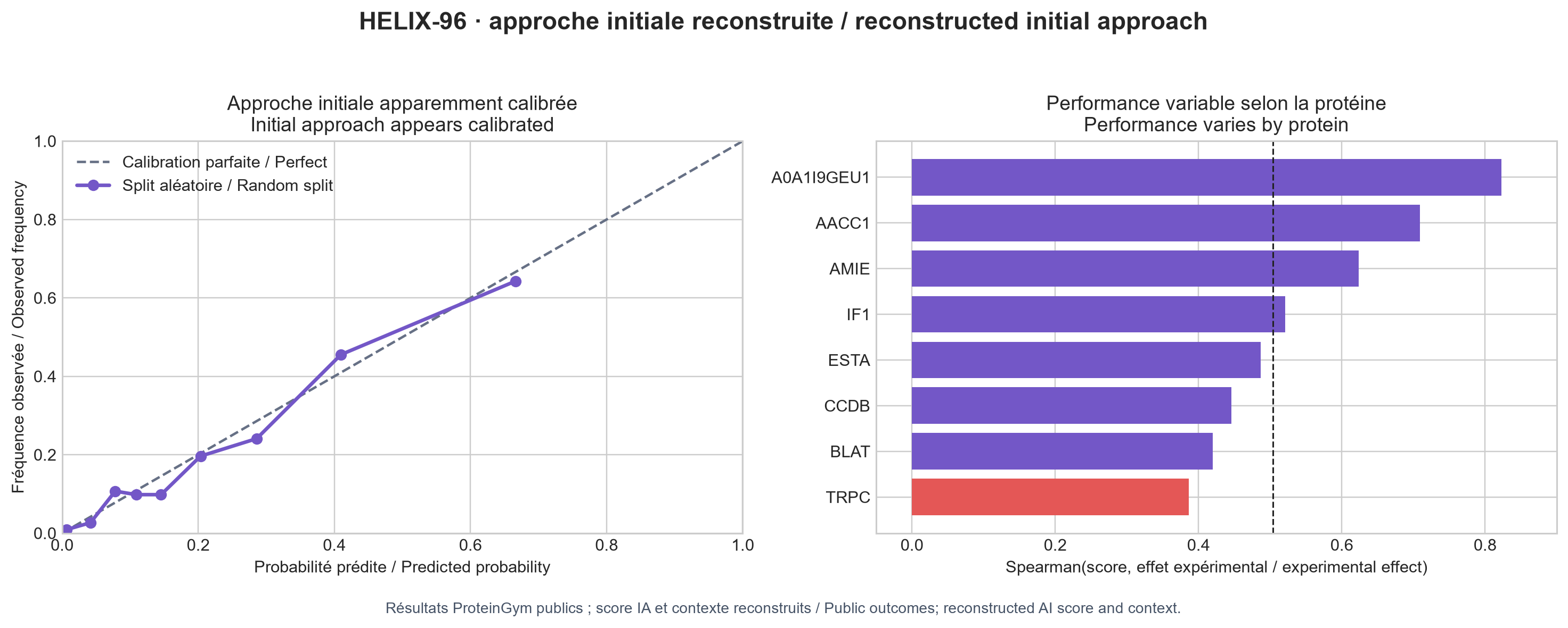
Random validation of the initial approach
The figure has two non-temporal panels. On the left, the horizontal axis is predicted probability and the vertical axis observed beneficial frequency, both from 0 to 1. Each purple point groups variants with similar predicted probabilities; the dashed grey diagonal is where prediction and frequency would match. On the right, the horizontal axis is the unitless Spearman rank correlation between score and experimental effect, and the vertical axis lists proteins. Each bar measures ranking quality for one protein; bars are purple except TRPC, highlighted red as the weakest case, and the dashed vertical line marks the median near 0.50.
On the left, points look broadly close to the diagonal under random splitting. On the right, correlation nevertheless ranges from about 0.39 for TRPC to 0.82 for A0A1I9GEU1, with only four proteins above the median. We can conclude that reassuring aggregate calibration can coexist with highly uneven transfer across proteins. We cannot conclude that the model predicts a new protein: the left panel mixes already-seen proteins and no bar provides an uncertainty interval.
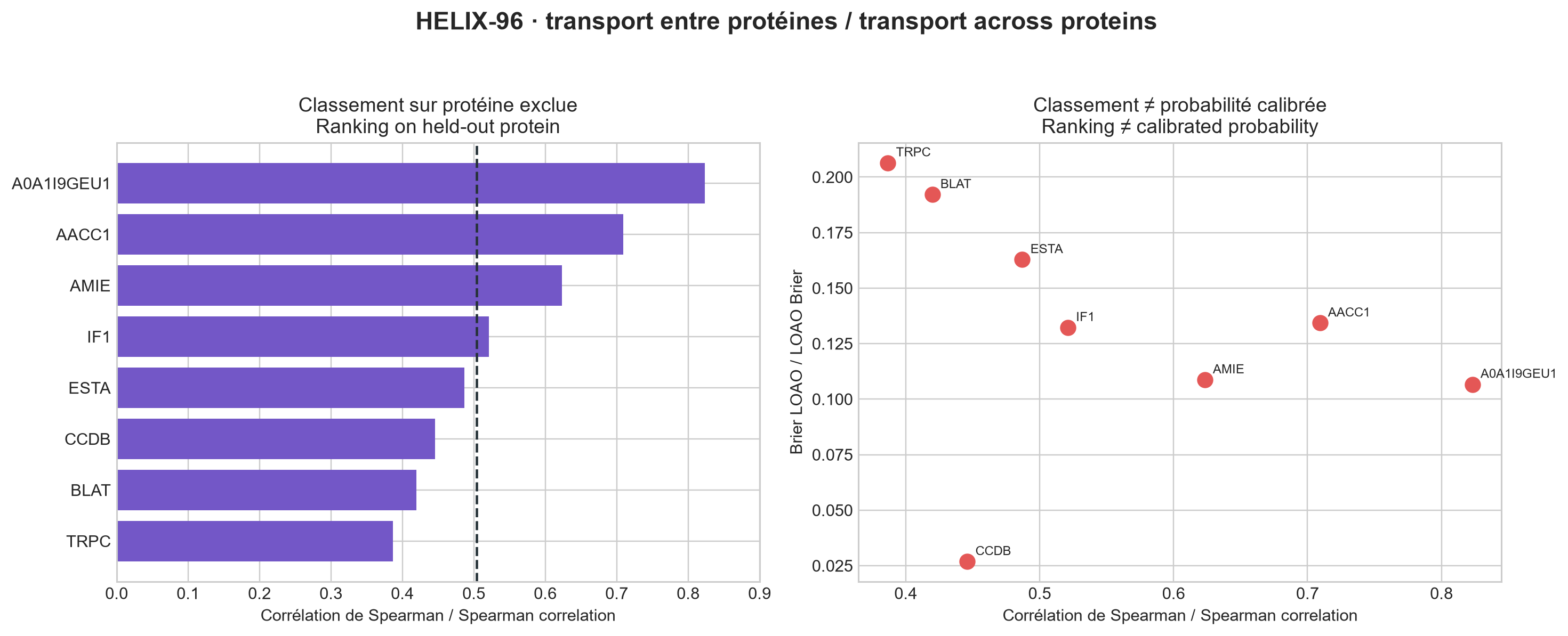
Score performance by biological experiment
In the left panel, the horizontal axis is unitless Spearman correlation and the vertical axis lists the eight proteins. Each purple bar measures whether the score ranks variants in the same order as experimental effect when that protein is held out; the dashed 0.50 line is a reference. The right panel again uses Spearman correlation horizontally and leave-one-assay-out Brier score vertically; the lower a red point, the better its calibration. Each labelled point therefore combines ranking quality horizontally and probability error vertically for the same protein.
A0A1I9GEU1 combines correlation near 0.82 with Brier score around 0.106; CCDB ranks less well, around 0.45, but has the best Brier score, about 0.027; TRPC is weak on both axes, around 0.39 and 0.206. We can conclude that good ranking and good calibration are distinct qualities, and that no single performance number summarises all eight groups. We cannot choose a universal threshold from this dispersion or interpret these points as clinical or human effects.
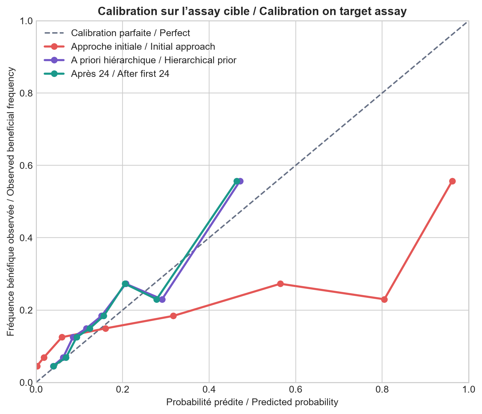
Probability calibration on the target group
The figure has one panel. The horizontal axis is predicted beneficial probability and the vertical axis observed beneficial frequency, from 0 to 1. Each point groups variants with similar probabilities; a point on the dashed grey diagonal would be perfectly calibrated. Red is the initial approach, purple is calibration with hierarchical information before the target experiment, and dark teal is the update after the first 24 experimental wells. Calibration error is read as the vertical distance between a coloured point and the diagonal at the same stated probability.
The red line is strongly overconfident in its high-probability bins: near a stated 0.95, observed frequency is only about 0.55. Purple and dark teal move much closer to the diagonal and the hierarchical correction reduces Brier score from 0.215 to 0.141; the two corrected lines almost overlap. We can conclude that the main correction improves probability coherence, while the first 24 outcomes add almost no further gain here. We cannot conclude that calibration will hold on new data because construction remains retrospective and points are group averages, not individual guarantees.
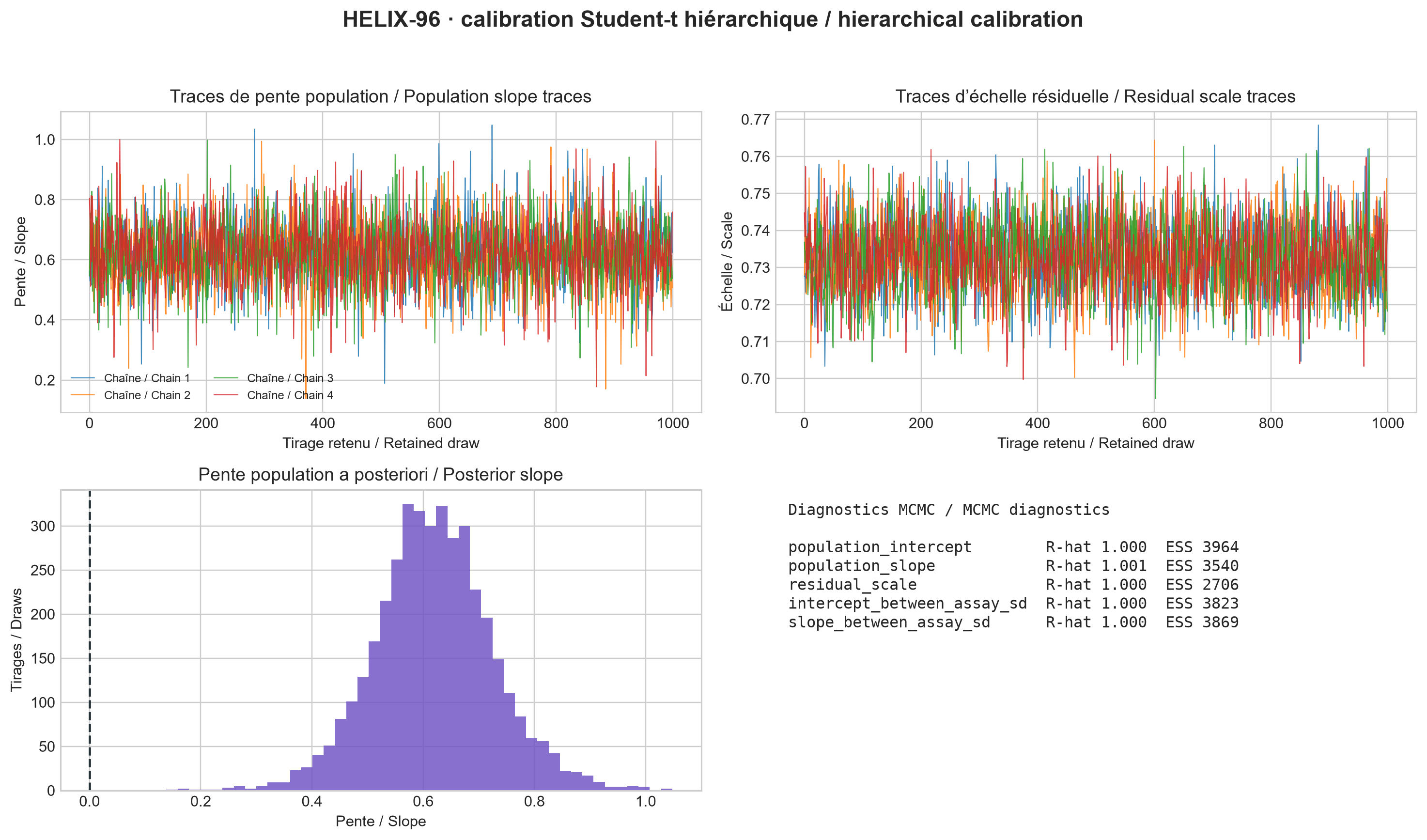
Diagnostics for the four computational chains
The figure has four panels. In the upper left, the horizontal axis counts 1,000 retained draws and the vertical axis gives population slope; in the upper right, the same horizontal axis accompanies residual scale vertically. The blue, orange, green and red lines are four independent computational chains; a point is one chain's value at a given draw. In the lower left, the horizontal axis again shows possible slope values and the vertical axis counts draws in each purple histogram bar; the dashed line marks zero. The lower-right panel is an axis-free diagnostics table reporting R-hat and effective sample size for five parameters.
The four traces overlap without visible drift, posterior slope is centred near 0.6 and most of its histogram remains above zero. Maximum R-hat is 1.00058 and minimum effective sample size is 2,706, with other sizes approaching 4,000. We can conclude that chains converged to the same numerical distribution and that a useful number of draws remains after accounting for correlation. We cannot conclude that the biological model is true, that data are sufficient or that the slope predicts new experiments: these diagnostics test computation, not external scientific validity.
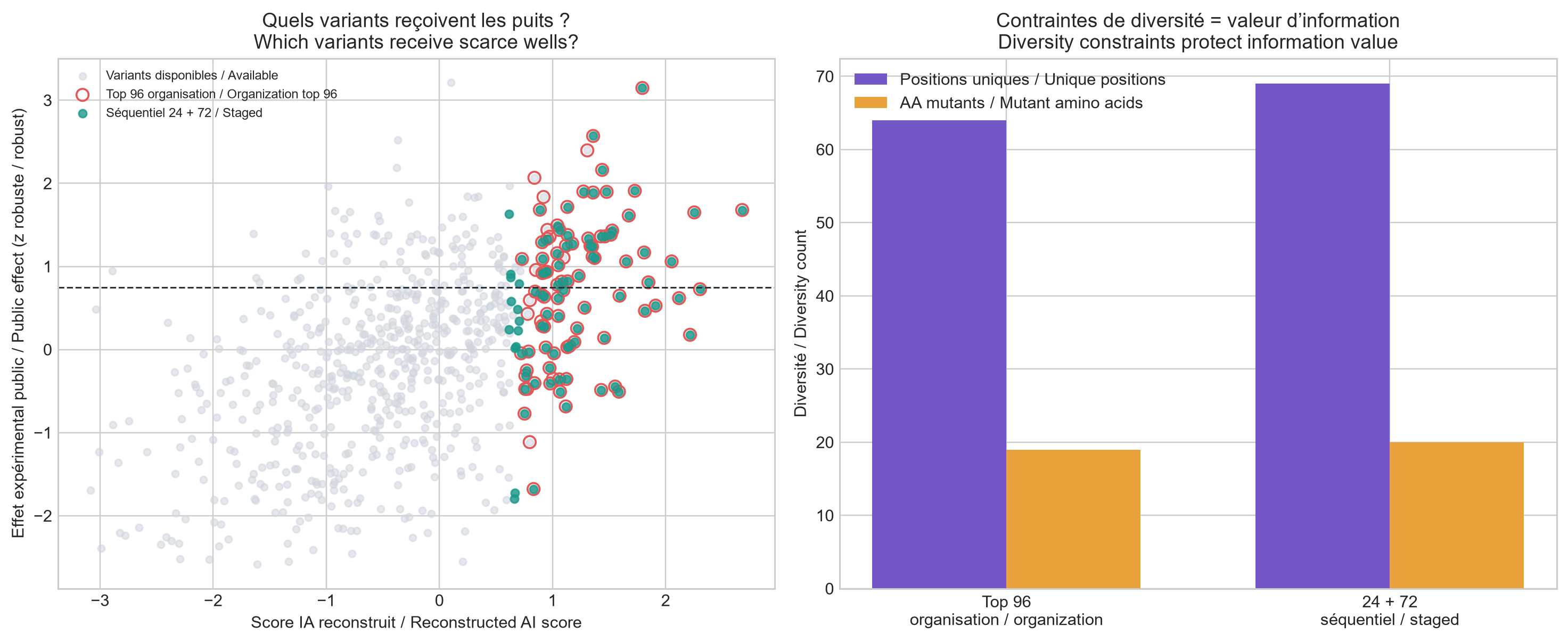
Positive results and diversity across the two lists of 96 variants
The figure has two panels. On the left, the horizontal axis is reconstructed AI score in standard deviations and the vertical axis is public experimental effect, also standardised. Each pale-grey dot is an available variant; hollow red circles mark the organisation's 96 choices and dark-teal dots the staged 24 + 72 choices. When a green dot has a red ring, both plans selected the same variant. The dashed horizontal line near 0.75 is the beneficial-outcome threshold used in this reconstruction. On the right, the horizontal axis compares the two plans and the vertical axis counts diversity: purple bars are unique protein positions and orange bars unique mutant amino acids.
The organisation's plan covers 64 positions and 19 mutant amino acids; the staged plan covers 69 and 20. The left-hand cloud shows both lists concentrating on high scores while public effects remain widely dispersed, sometimes below the threshold. We can conclude that the staged constraint modestly broadens list diversity in this reconstruction. We cannot conclude that diversity alone produces more positive outcomes or that the score would be available with the same quality before a new experiment: the displayed effects are already known.
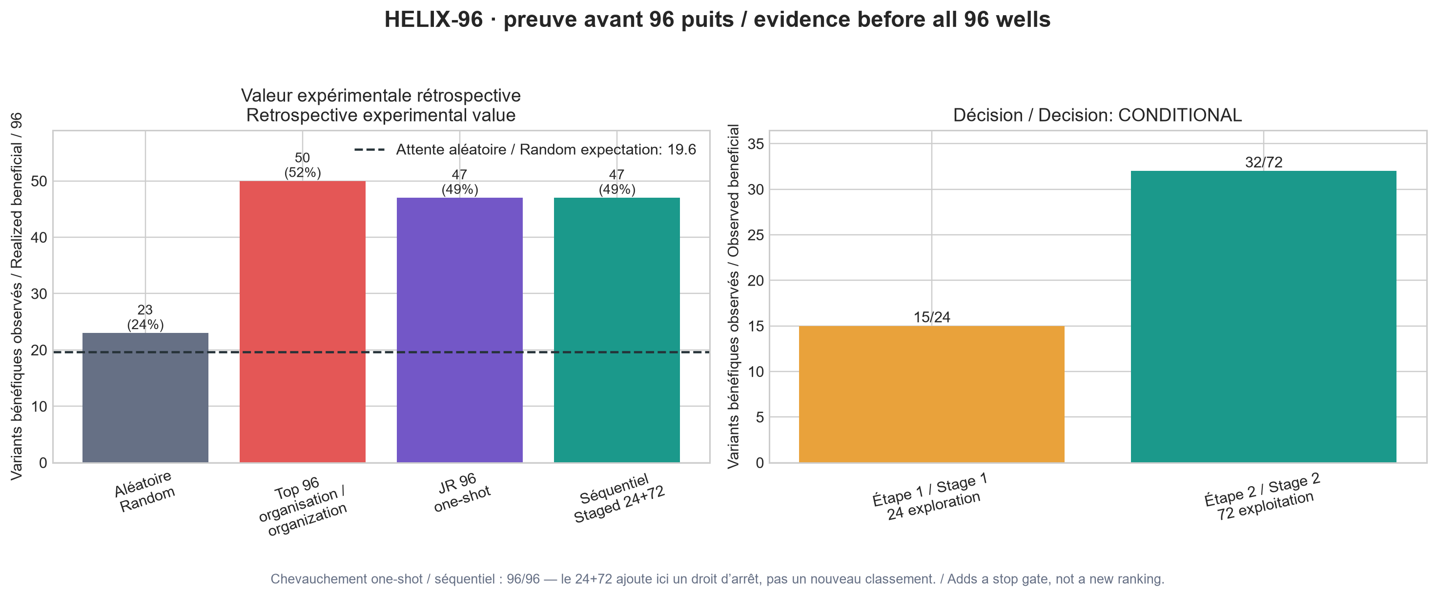
Decision value of the 24-plus-72 plan
The figure contains two count panels. On the left, the horizontal axis compares four selection methods and the vertical axis counts observed beneficial variants out of 96; the dashed 19.6 line is the random-selection expectation. Grey, red, purple and dark-teal bars give 23 of 96, 50 of 96, 47 of 96 and 47 of 96 respectively; each height is an outcome count and its percentage is printed above. On the right, the horizontal axis separates the 24-well exploratory stage from the following 72-well stage, while the vertical axis counts beneficial outcomes: 15 of 24 in orange, then 32 of 72 in dark teal.
Both corrected methods total 47 beneficial outcomes; the two-stage plan simply decomposes that total into 15 + 32 and permits a decision after the first 24 wells. The initial approach shows 50, three more, but the preceding figure shows lower diversity. We can conclude that, in this retrospective implementation, staging creates a right to stop but neither a new final ranking nor an outcome gain. We cannot infer that stopping would actually have occurred, that 47 or 50 would be reproduced on new data, or that the three-outcome gap is statistically significant.
07 · Assessment protocol
How the assessment was conducted
Assessment protocol
- Eight public ProteinGym experiments, with 700 mutations each.
- Robust hierarchical statistical model, four computational chains and 4,000 retained draws.
- Maximum R-hat diagnostic: 1.00058; minimum effective sample size: 2,706.
- The eighth group is held apart; calibration is measured before and after the first 24 experiments.
Limitations that matter
- The AI score is reconstructed from public outcomes and is not a prediction on future data.
- The first 24 results are evaluated retrospectively.
- Brier score deteriorates slightly after the 24-well update.
- Biologically heterogeneous assays; no clinical, patient or human outcome.
08 · Sources & provenance
Where the facts come from
09 · Decision
CONDITIONALCONDITIONAL — improved calibration, but no ranking gain or blind export from a real model.
- 1
Hierarchical calibration improves the Brier score on the target, but this analysis reconstructs the score from outcomes already known.
- 2
The corrected selection obtains three fewer positive results while covering more positions. The 24 + 72 plan changes none of the 96 choices here.
- 3
The next step requires a real score frozen before the experiment, a pre-written stop rule and validation on new outcomes.
Next step: Proceed only with a frozen real score, a stop rule written before the experiment and future validation under real conditions. Here, the selection made entirely upfront and the two-stage plan retain exactly the same 96 variants.