Industrial compute capacity
Estimating the future cost of compute capacity, defining what could actually be traded, and showing why a credible market requires telemetry, forecasting and verifiable delivery.
Organization, parameters and data are entirely reconstructed. Calculations, simulations and charts were genuinely executed.
Synthetic dataReading plan
From problem to decision
- 01
Define the objects
Distinguish future cost, expected average, forward value and contractual payoff.
- 02
Reconstruct the prototype
Follow mean reversion and then the Black-76 valuation step.
- 03
Audit the assumptions
Correct convexity, separate forecasting from valuation, then verify the calculation by simulation.
- 04
Measure fragility
Test stress regimes and the ability of data to identify parameters.
- 05
Design a testable market
Standardise the traded capacity, forecast supply and demand from telemetry, then organise delivery.
- 06
Form a decision
State what can be kept, rejected or replaced before any use.
01
Before we begin
The problem
A reconstructed organization wants to represent hourly costs for three synthetic generations of compute capacity, then value a contract granting the right, but not the obligation, to buy that capacity at a predetermined price. The next objective is to turn that idea into a testable market backed by genuinely deliverable capacity.
This reconstructed study examines a concrete industrial problem: representing the possible evolution of the cost of one hour of compute, then valuing a contract that grants the right—but not the obligation—to buy that capacity at a predetermined price.
Three synthetic generations, named A, B and C, are used to study different cost profiles. One accelerator-hour means using a processor specialised in intensive computation for one hour. These generations are neither real products nor observed market prices. Parameters are synthetic; calculations, simulations and charts are genuinely executed.
The improvement objective extends beyond mathematical correction: it also requires defining how compute capacity could be traded. The cost model is only a first building block; a standard unit, supply-and-demand forecasts and verifiable delivery are still required.
02
Phase 1
What the organization built
We begin by understanding the system as presented, without caricaturing it and before proposing any correction.
The service the prototype seeks to represent
The starting quantity is Sₜ: the cost, at future time t, of one hour of compute capacity. The prototype does not assume that this cost drifts freely forever; it assumes that its logarithm gradually returns towards a long-run level.
This mechanism is described by an Ornstein–Uhlenbeck process. It can represent the economic idea that scarce capacity becomes expensive, attracts supply, then moves towards a more sustainable level. That intuition remains a hypothesis to test, not a fact established by synthetic data.
The prototype's central curve
The prototype first calculates the theoretical average of log cost, then applies the exponential function. The resulting quantity, exp(E[log Sₜ]), is the median cost in the model: half the scenarios lie above it and half below.
The problem appears when this median is called expected average cost. The exponential function is convex: large upward scenarios increase the average more than comparable downward scenarios reduce it. A variance term is therefore missing from the initial formula.
From future cost to the value of a purchase right
The studied contract allows its holder to buy one hour of capacity at an agreed strike price. If future cost exceeds that price, the right has value; otherwise, its holder may leave it unexercised.
The prototype uses the central curve as a forward value, converts variance into annual volatility, then applies Black-76. The chain produces a number, but this does not prove that its curve is an observable forward value or that the lognormal distribution required by the formula is suitable.
Initial approach summary
- The prototype makes log cost gradually revert towards a long-run level.
- It displays the exponential of average log cost as its central curve, then treats it as a forward value.
- It finally applies the Black-76 formula to value a purchase right, without separating historical forecasting from valuation assumptions.
03
Phase 2
What the assessment checks and proposes
The second phase reproduces the mechanism, locates what breaks and turns criticism into a testable change.
Correct the average before discussing price
The audit starts by naming each object. When log cost is normal, expected average cost equals exp(mₜ + vₜ/2), where mₜ is mean log cost and vₜ its variance. The initial exp(mₜ) curve omits vₜ/2.
For generation B near eighteen months, this correction places expected average cost 7.49% above the initial curve. This gap is an internal consequence of the equations; it does not measure error against a real market.
Separate historical forecasting from valuation
The historical distribution seeks to describe the frequency of future scenarios. The valuation distribution answers another question: what weight should those scenarios receive today when valuing a contingent payment? The two must not be conflated.
The corrected model links them through a disclosed price of risk. This relationship is an assumption. If compute capacity cannot be bought, sold and hedged in a liquid market, it does not automatically follow from a no-arbitrage argument.
Verify the calculation without claiming to validate the world
A Monte Carlo simulation generates 120,000 terminal costs under the same model, then calculates their average. It obtains 3.0392 dollars per hour versus 3.0377 for the corrected analytical formula, a 0.0508% relative gap.
This proximity shows that the simulation code and formula implement the same assumption. It proves neither that the synthetic parameters are realistic nor that the Ornstein–Uhlenbeck process describes future prices.
Test regimes and identification
The purchase right is then revalued under two regimes: a frequent calm regime and a rare but more dispersed stress regime. Even when mean and variance are close, the shape of extreme scenarios changes contract value. The relative gap reaches 8.82% over the tested grid.
Finally, the audit asks whether one or five years of weekly data are sufficient to recover mean-reversion speed and long-run level. A broad parameter region remains almost equally compatible with the simulated path: the model is weakly identified.
Define what would actually be traded
One graphics processor is not interchangeable with every other one: generation, memory, interconnect, location and availability change the delivered service. The proposed product is therefore not ownership of a physical machine, but a standardised capacity block. Each block specifies accelerator class, the minimum number of accelerators that can be used together, site or region, start window, duration and availability commitment.
The first mechanism would be a sealed double-sided day-ahead auction. Each data centre submits a firm quantity and minimum price for its blocks; each buyer submits a quantity and maximum price. Seller offers are ranked from lowest to highest, buyer bids in the opposite order, and pairs are matched while the buyer maximum covers the seller minimum. A published rule sets one uniform price between the two accepted marginal prices. The reservation is then delivered through the data-centre scheduler. Dedicated metering reconciles scheduler logs with telemetry; a monitoring dashboard alone is not sufficient for financial settlement.
Once several months of reliable deliveries and prices exist, a forward contract can fix today the price of a block delivered later. An optional purchase right would come only afterwards: without delivery history, an observable forward curve and a way to manage risk, applying Black-76 directly amounts to valuing a market that does not yet exist.
Forecast supply and demand from data centres
Supply is not simply the number of installed processors. At each horizon, already committed reservations, planned maintenance and an incident buffer must be subtracted from healthy capacity. Internal telemetry must therefore track health, utilisation, memory, accelerator-to-accelerator communication, power, temperature and outages; the scheduler adds reservations and jobs already allocated.
Demand is visible in the queue, but also in rejected or abandoned requests: accelerator class, number of processors that must run together, estimated duration, deadline, start-time flexibility, cancellations and interrupted jobs. The ratio of requested accelerator-hours to net available capacity measures expected pressure. The forecasting layer uses only anonymised aggregates by class, region and time bucket. A restricted contractual layer nevertheless retains verified identity, safeguards, limits and delivery history under a stable identifier; neither those identities nor workload contents are published.
The forecast must produce a distribution, not one point: shortage probability, utilisation range and price range for the next twenty-four hours, then for the week and month. It is replayed chronologically against a simple seasonal baseline. Quality is judged by probability calibration, volume error, delivery failures and the gap between forecast and actual clearing prices.
Learn first in a shadow market
Deployment would start with twelve weeks and no financial exchange. Suppliers would publish the blocks they believe they can deliver, buyers would submit intentions pseudonymised for analysis, and the engine would calculate allocations and prices as if the auction were real. The restricted registry would retain verified identities so that concentration and per-participant limits could be measured. Capacity would continue to be managed normally; simulated decisions would then be compared with reservations, utilisation and incidents actually observed.
Before the pilot, acceptance thresholds would be fixed for telemetry completeness, forecast calibration, delivery rate, participant concentration and the gap between the reference index and the service actually received. One severe failure—manipulable data, unverifiable delivery, dependence on a single participant or an unvalidated legal framework—would keep the decision at NO-GO.
If the shadow market is successful, the progression would be: day-ahead auction with payment safeguards, physically delivered forward contracts, and only then optional purchase rights. This sequence creates the observations missing from the current model instead of assuming that a liquid market already exists.
Assessment
- For generation B at about eighteen months, expected average cost is 7.49% above the initially displayed curve.
- A 120,000-scenario simulation reproduces the corrected formula within 0.0508% relative error.
- The single-volatility formula deviates by up to 8.82% from the tested regime mixture, while several parameters remain almost equally compatible with five simulated years.
- The prototype does not yet measure net available capacity, future demand or delivery quality; by itself, it therefore cannot form a capacity market.
Proposed correction
- Restore the variance term that turns a median into expected average cost.
- Explicitly separate the historical distribution from the distribution chosen to value the contract.
- Compare the single-volatility formula with a mixture containing calm and stress regimes.
- Expose simulation verification, model risk and weak parameter identification.
- Define a deliverable contractual block: accelerator class, number of processors that can run together, region, window, duration, interconnect and availability level.
- Connect healthy capacity, commitments, maintenance and queues to signed telemetry; forecast supply, demand and shortage probability separately.
- Test a shadow market first, then a physically delivered day-ahead auction and forwards; consider options only after observing a reliable underlying market.
04
Concepts and equations
No symbol without a definition
The same notes open from the “?” links placed throughout the article.
05
Numerical results
What the numbers actually measure
These numbers assess internal consistency and sensitivity of the synthetic model. They are neither observed prices nor market forecasts. Without operational telemetry, this version does not yet calculate any supply or demand forecast.
generation B convexity gap
Difference between corrected expected average cost and the displayed median near eighteen months.
simulation error
Relative gap between 120,000 scenarios and the corrected analytical formula.
maximum option gap
Largest relative gap between the single-volatility formula and regime mixture over the tested grid.
grid needed for 90% of weight
A large share of the grid remains compatible with five simulated years: identification remains weak.
06 · See the evidence
Read the charts step by step
Each figure first explains how to read its axes and colours, then what it does—or does not—support.
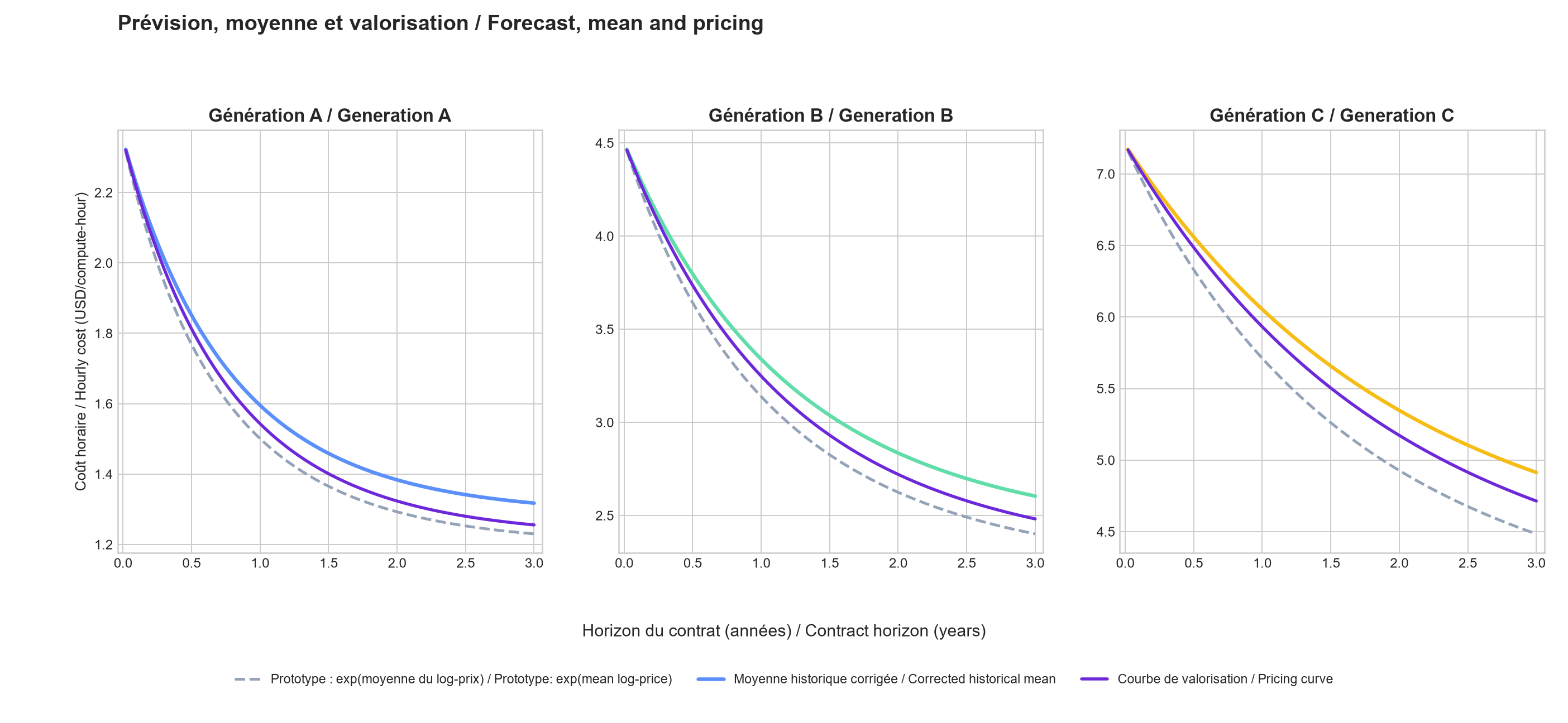
Comparison of medians, expected average costs and valuation values for three compute-capacity generations
The three panels show generations A, B and C from left to right. In each, the horizontal axis is the 0-to-3-year horizon and the vertical axis is cost in dollars per accelerator-hour. Dashed grey is the prototype median; the blue, mint-green or yellow line is expected average cost under historical dynamics; purple is the value used to price the contract. At a given maturity, read the three heights vertically in the same panel: their separation reflects different definitions, not three competing observations.
For generation B near eighteen months, median, expected average cost and the valuation curve are about $2.825, $3.037 and $2.930 per hour. We can conclude that conflating these three quantities materially changes the contract-pricing input. We cannot conclude that the purple curve is tradable or correct: the median-to-mean gap follows from model algebra, while the valuation gap depends on an assumed, unobserved price of risk.
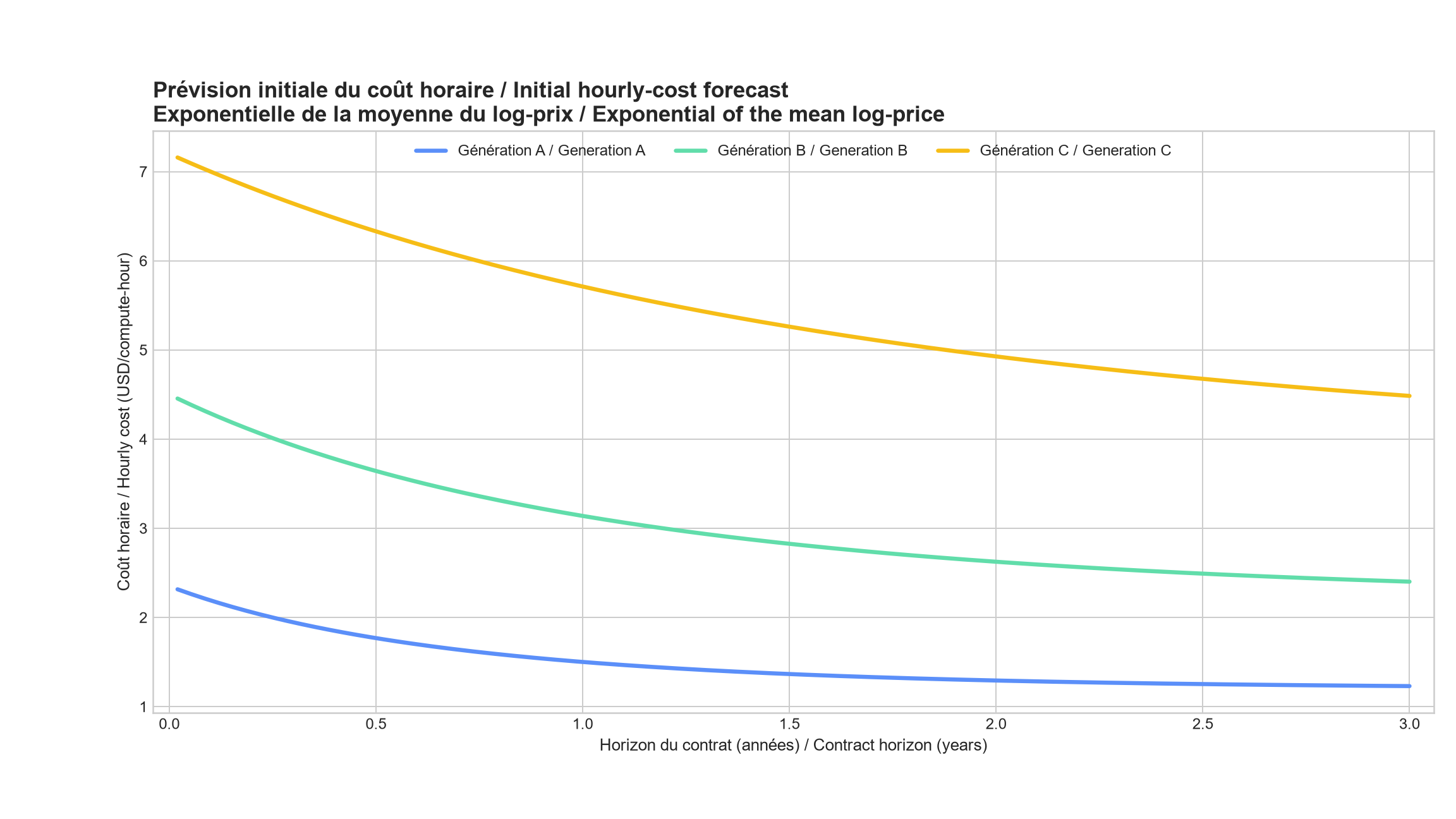
Medians modelled by the initial prototype for three compute-capacity generations
The figure has one panel. The horizontal axis is contract horizon, from 0 to 3 years; the vertical axis is a synthetic hourly cost in US dollars per accelerator-hour. The blue, mint-green and yellow lines represent generations A, B and C respectively. To read a line, choose a maturity on the horizontal axis and move upward to the required colour: its height is the prototype's median cost at that maturity.
The medians fall from about $2.32 to $1.25 for A, $4.45 to $2.40 for B and $7.15 to $4.48 for C between inception and three years. We can therefore conclude that the chosen mechanism imposes gradual reversion towards a long-run level. We cannot conclude that these levels will be the average costs actually paid or that they are observed forward prices: data and parameters are synthetic, and a median is not a mean.
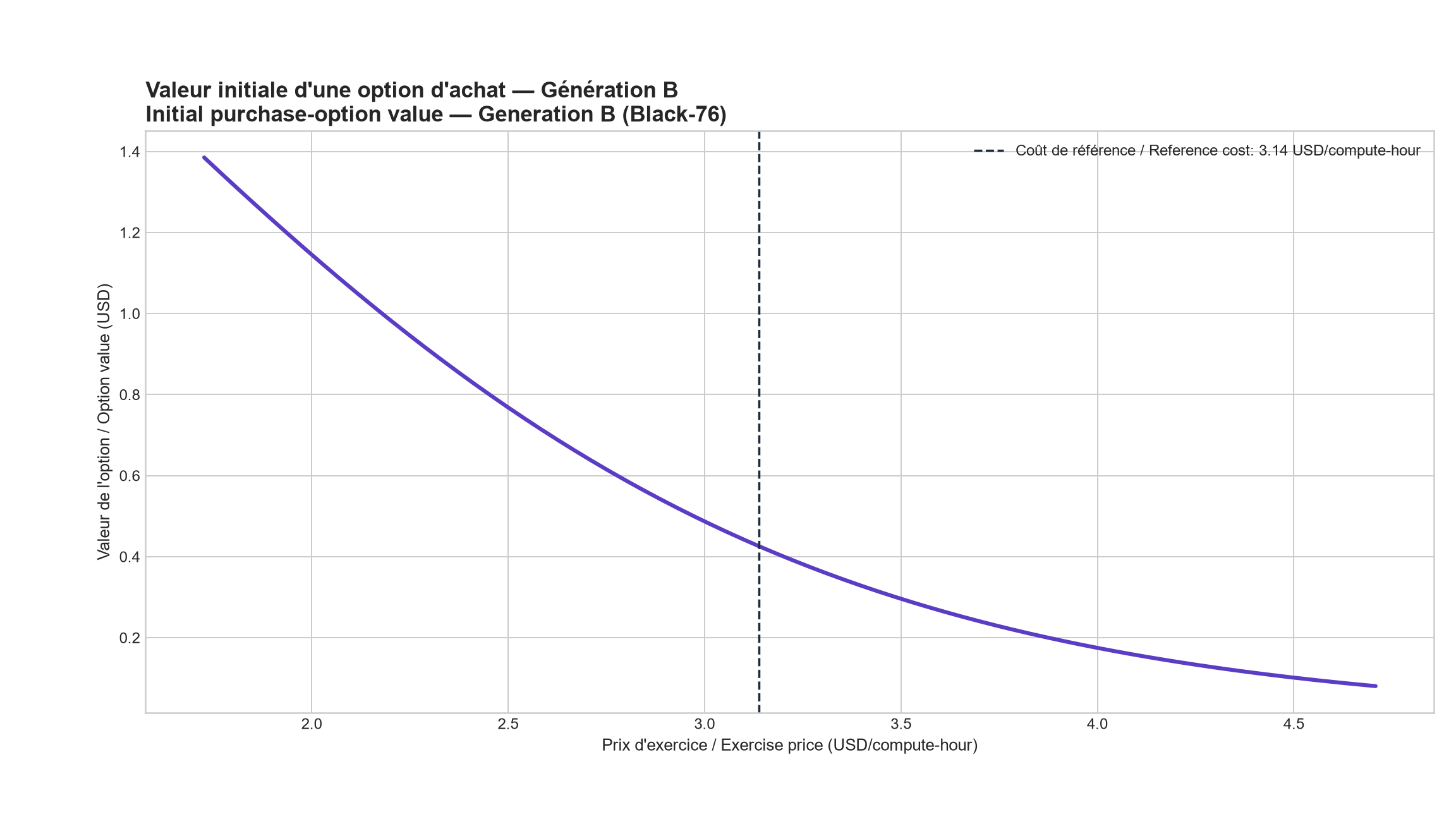
Purchase-right value calculated with Black-76 in the initial prototype
The figure has one panel for generation B. The horizontal axis is contractual exercise price in dollars per accelerator-hour; the vertical axis is the discounted purchase-right value in dollars. The purple line gives one value for each exercise price. The vertical dashed line marks the $3.14 reference hourly cost: where it meets the curve, the right is worth about $0.43.
Value falls from about $1.38 at an exercise price near $1.7 to less than $0.10 near $4.7. We can conclude that the calculation respects the minimum intuition for a purchase right: a higher exercise price makes it less valuable. We cannot infer that $0.43 is a fair market price, because the forward curve, volatility, rate and, above all, the suitability of Black-76 have not been calibrated to a liquid market.
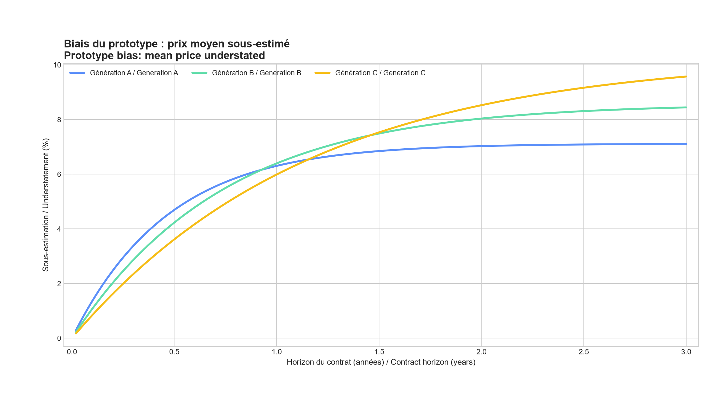
Convexity gap between the initial curve and corrected expectation
The figure has one panel. The horizontal axis is contract horizon from 0 to 3 years; the vertical axis is mean-cost understatement in percent when the prototype uses the exponential of mean log cost. Blue, mint-green and yellow correspond to generations A, B and C. Read a point as follows: at the selected maturity, its height is the percentage that must be added to the prototype median to recover the mean under the same model.
Near eighteen months, generation B's gap is 7.49%. At three years the lines reach roughly 7.1% for A, 8.4% for B and 9.6% for C. We can conclude that omitting the variance term creates a bias that grows with horizon. We cannot call this a real forecasting error: both quantities are calculated within the same synthetic model and have not been compared with observed costs.
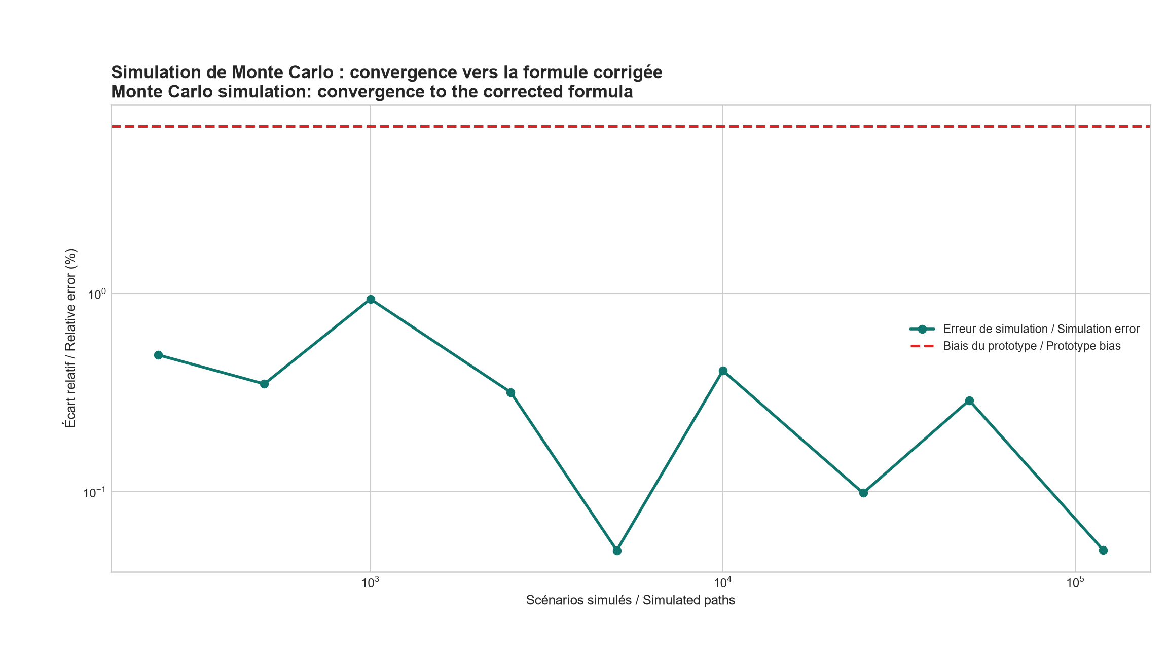
Simulation verification of expected average cost for generation B
The figure has one panel and both axes are logarithmic: equal spacing represents multiplication, not constant addition. The horizontal axis is the number of simulated paths; the vertical axis is absolute deviation from the corrected formula in percent. Each dark-teal point is an estimate at a given path count, and the line merely connects those runs. The dashed red line near 7.5% recalls the persistent bias in the initial prototype.
The green-point error fluctuates because simulation remains random, but it falls below 0.1% for some large samples and equals 0.0508% with 120,000 paths, far below the red line. We can conclude that the simulation code converges to the corrected formula. We cannot conclude that the formula describes reality: Monte Carlo is checking an implementation against its own model, not the parameters or economic distribution.
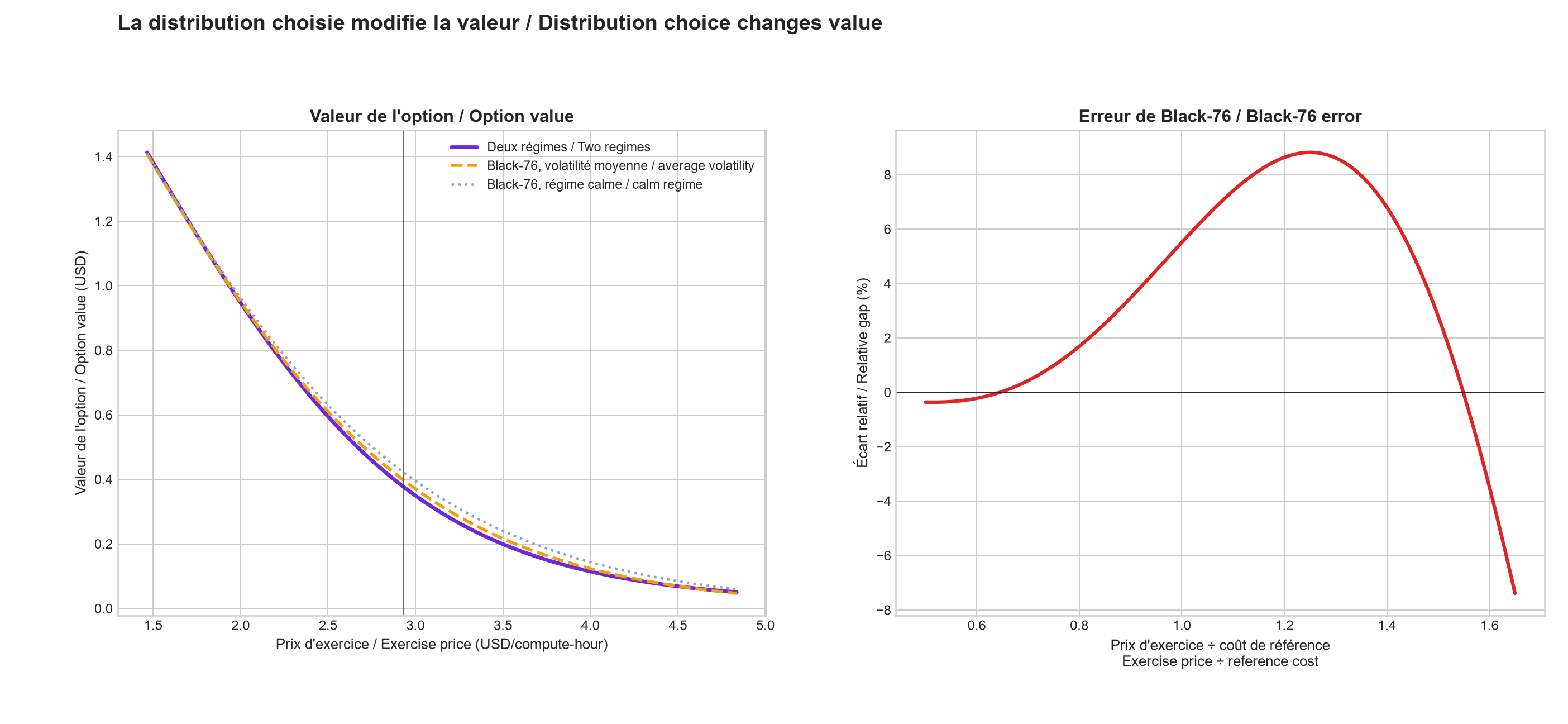
Option-price gap between Black-76 and a regime mixture
In the left panel, the horizontal axis is exercise price in dollars and the vertical axis is discounted purchase-right value in dollars. Purple is the two-regime model, dashed orange is Black-76 with average volatility and dotted grey is Black-76 using only the calm regime; at a given exercise price, their heights give three valuations. In the right panel, the horizontal axis is exercise price divided by reference cost and the vertical axis is Black-76's relative gap to the two-regime model in percent; the red line exposes the gap hidden by the overlap on the left.
On the left, all values fall from about $1.4 to less than $0.1 as exercise price rises. On the right, the gap peaks at 8.82% around a ratio of 1.25 and even changes sign at the grid extremes. We can conclude that models that nearly overlap in dollars can differ materially in relative terms, especially for some payoff regions. We cannot conclude which is correct without tail data, nor treat the maximum gap on this grid as a guaranteed market-pricing error.
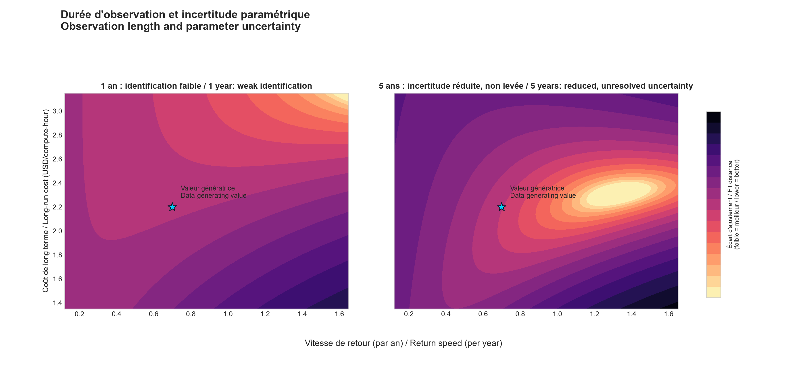
Likelihood surfaces for Ornstein–Uhlenbeck process parameters
The left panel uses a one-year path and the right a five-year path. In both, the horizontal axis is return-to-long-run speed per year and the vertical axis is the long-run level in dollars per accelerator-hour. Each map location is therefore one parameter pair. Colour measures distance from best fit: pale yellow is better, purple and then black worse. The cyan star marks the synthetic pair that generated the data, about 0.7 per year and $2.2.
After one year, a broad band of pairs gives similar fits; after five years, a pale region emerges but remains wide, and its best point does not exactly coincide with the star on this particular path. Overall, 70.5% of the grid is still required to contain 90% of relative weight. We can conclude that more observations reduce ambiguity without cleanly identifying both parameters. We cannot conclude that the pale region provides reliable estimates for real data: this is one synthetic path with no out-of-sample test.
07 · Assessment protocol
How the assessment was conducted
Assessment protocol
- Ornstein–Uhlenbeck process applied to log cost across three synthetic generations.
- Historical and valuation distributions separated through an explicit risk-price assumption.
- 120,000 terminal Monte Carlo scenarios, random seed 20260811.
- Single-volatility Black-76 compared with a calm-stress lognormal mixture.
- Likelihood surface over mean-reversion speed and long-run level.
- Proposed, unexecuted improvement architecture: standardised block, supply-and-demand telemetry, probabilistic forecasting, shadow market and physical delivery.
Limitations that matter
- No price history, order book or quoted option data.
- Ornstein–Uhlenbeck parameters, risk prices and regime mixture are chosen rather than estimated.
- Monte Carlo checks the formula inside the same model; it does not validate the model against reality.
- One identification path and no out-of-sample test.
- No data-centre telemetry, job queue, reservation, failure, power constraint or rejected demand is yet observed.
- No market pilot, clearing price, contractual delivery, financial safeguard or legal analysis has been executed.
08 · Sources & provenance
Where the facts come from
- Synthetic data and parameters generated by the reproducible package
- NVIDIA DCGM — accelerator telemetry and Prometheus exporter
- Slurm — queues, requested resources and job state
- Slurm — accelerator utilisation and memory accounting
- Prometheus — time-series monitoring and limits for exact billing
- AWS EC2 Capacity Blocks — public example of future accelerated-capacity reservation
09 · Decision
REVISEREVISE — the mathematical correction works, but the parameters and valuation method are not yet operationally defensible.
- 1
The prototype correctly illustrates return towards a long-run level, but conflates a median, expected average cost and a valuation input. This confusion must be corrected before any decision.
- 2
The corrected average formula is numerically verified. However, parameters remain weakly identified and purchase-right value is materially sensitive to the chosen distribution.
- 3
Before use, the service and contract must be precisely defined, traceable series collected, estimation uncertainty disclosed and out-of-sample tests performed.
- 4
Moving to trading requires a layer absent from the prototype: a standardised block, aggregated data-centre telemetry, probabilistic supply-and-demand forecasts, then verifiable delivery that prevents the same slot from being sold twice.
- 5
The next defensible experiment is a shadow market. A live auction can start only after chronological validation of data, forecasts, settlement, safeguards, concentration and the legal framework. Under the cautious protocol proposed here, forward contracts must be validated before an option is tested.
- 6
If no liquid hedge justifies Black-76, the formula should be rejected in favour of expected-cost scenarios with an explicit risk premium. If mean reversion remains weakly identified, a simpler curve with robust intervals is preferable. If the lognormal distribution fails stress tests, the regime mixture or direct simulation should replace the approximation.
Next step: Revise before operational use. The first step is not to quote an option: define a deliverable unit, instrument supply and demand, then run a twelve-week shadow market. A live auction, forwards and finally options become admissible only after chronological validation of telemetry, forecasts, delivery, safeguards and the legal framework.